by John Donald, Lecturer, School of Accounting, Economics and Finance, Deakin University, Australia
In the last instalment of Student Notes we looked at the balenciaga scarpe uomo various behaviour patterns that costs can exhibit. These patterns are important because knowledge of them can enable predictions of future cost amounts and also the use of decision-making techniques like cost-volume-profit analysis and flexible budgeting. When there are semi-variable (or mixed) costs we need to be able to determine how much of each one is fixed and how much is variable. We also need to know how the variable component of such a cost will change in response to changes in the principal cost driver. This set of Student Notes describes the methods which can be used to analyse (or estimate) cost behaviourpatterns and thus enable the prediction of future costs. We will also consider the problemsassociated with the different cost estimation methods that can be used. Cost estimation
This is the process of determining how a cost changes in relation to variations in a particular cost driver or, in some cases, with variations in multiple cost drivers. The aim of this process is to establish a numerical relationship between a cost and the main factor which causes the cost to be incurred.Such a factor is called the root cause cost driver. This may be an activity which is carried out as part of the production process, or it may be some input which is needed for a particular production activity. For example, an assembly labour cost for a given time period may vary with the number of units assembled during that period. Likewise, for a bakery the cost of electricity consumed may vary with the number of batches of bread baked. The number of units assembled and the number of batches baked are cost drivers which are output measures. However, if batches of different breads take different times to bake in an electric oven, the cost of electricity will vary, not with the total number of batches baked, but with the total number of kilowatt-hours of electricity consumed.This type of cost driver is an input measure. To be able to predict future costs accurately there should be a strong correlation between a cost and the chosen cost driver, but we also need to be able to predict future changes in the cost driver easily.
Non-quantitative methods of cost estimation
Cost estimation methods can be either nonquantitative (based on skilled judgement) or quantitative (based on a mathematical analysis of past cost data). Non-quantitative methods include:
(i) The industrial engineering method (sometimes called the work measurement method). This method can be used by both manufacturing and service organisations for estimating costs and it involves studying the processes that cause costs to be incurred. The aim is to identify the relationships which should exist between inputs and outputs. Industrial engineers could conduct time and motion studies (or task analyses) which involve observing employees as they undertake work tasks and establish a normal time for each type of task. These balenciaga scarpe uomo times are then costed using the wage rates for the various types of worker. By analysing the sequence of tasks or activities needed to make a particular product or to provide a certain type of service, a normal or standard labour cost canbe estimated. The engineers can then determine from design specifications the types and quantities of material required for each unit of the product or service and how much these materials should cost. An estimated amount of overhead cost will be added to the material and labour costs and this gives a standard unit cost which can then be used to predict future costs based on planned levels of activity.
The industrial engineering method relies for its accuracy on the skills and experience of trained engineers. It is time-consuming and expensive, but it has to be used when estimating costs for a completely new product because there is no historical data to rely upon. This method is most useful for estimating the costs of repetitive processes where input-output relationships for material and labour are clearly defined.
(ii) The account classification (or account analysis) method. Using this method requires the management accountant to review past cost behaviour patterns as shown in the organisation’s ledger accounts and other accounting records. He or she will then use judgement and knowledge of operations to classify each cost as either fixed, variable or semi-variable. For example, it may be clear from an analysis of the ledger accounts
that direct-material cost is variable, equipment depreciation is fixed and utility costs are semivariable. This examination of historical records is combined with an assessment of the factors which may affect the different costs in the future. For those costs which have been identified as semivariable, the management accountant will need to use one of balenciaga scarpe uomo several more systematic methods to estimate the fixed and variable components. These methods (the high-low method and regression analysis) are discussed later when we look at
quantitative methods of cost estimation.
(iii) The visual-fit method. With this method, a simple diagram called a scattergraph is used to create what is called a ‘line of best fit’. A number of data points, with each one representing the past amount of a particular cost and the corresponding level of activity, are plotted on a pair of axes with the independent variable (a cost driver such as the number of units produced) on the horizontal or X-axis and the dependent variable (total cost
amount) on the vertical or Y-axis. The pattern of the plotted points helps the analyst to visualise the nature of the relationship between the cost amounts and the levels of the factor which is assumed to have caused the cost amounts i.e. the cost driver. It also enables the analyst to assess the strength of the relationship between the cost and the level of the assumed cost driver. If the relationship is fairly strong, the data points will fall
in a linear pattern i.e. they will resemble something close to a straight line. If, however, there is little or
no relationship, the data points will be more widely scattered with no obvious pattern . In this case, the
wrong cost driver may have been chosen.
If there does appear to be a relationship between a cost and the chosen cost driver, the analyst
can, by using judgement, draw a line of best fit through the data points so that approximately the
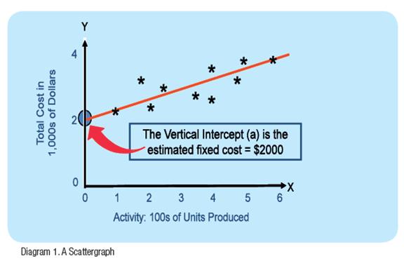
same number of points lie above and below it. This line represents the cost function Y = a + bX.
If the cost is semi-variable, the point where the cost line cuts the vertical or Y-axis (known as the
‘vertical intercept’) represents the estimated value of ‘a’ i.e. the fixed component of the cost. The
slope of the line represents the variable cost per unit of the cost driver i.e. the value of ‘b’in the
cost function. Diagram (1) below shows a typical scattergraph.
Scattergraphs are useful because they enable the analyst to identify quickly any outliers or abnormal data points. These are data points which do not conform to the same general pattern as the rest of the plotted points i.e. they represent cost or activity amounts which are unusually high or low. The analyst may decide to disregard these points when drawing a line of best fit and to omit them from any further analysis. Scattergraphs do provide an estimate of the fixed component of a semivariable cost but, as with the account-classification method discussed above, a quantitative method must be used to estimate the slope of the cost line (i.e. the value of ‘b’).
Quantitative methods of cost estimation http://www.sneaker2018.it/
(i) The high-low method.
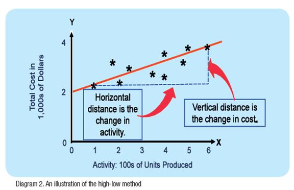
This method produces a cost function by using the highest and lowest activity (X) data points (hence the name ‘high-low’). It takes the change in cost between the highest activity level and the lowest activity level and divides this dollar amount by the corresponding change in activity to give an estimate of the slope of the cost line i.e. the variable cost per unit of activity (the value of ‘b’ in the cost function). Diagram (2) illustrates this process.
It is important to note that the high and low points are identified by looking at the activity levels and not the cost amounts. The period which had the highest cost may not be the period which had the highest level of activity.
As an example of how this method works, assume that we are trying to determine how the cost of electricity for a month changes with the number of machine hours worked during the month. The cost of electricity is usually semi-variable because the total dollar amount for a month will include a fixed supply charge plus a variable amount based on the number of kilowatt hours of electricity consumed. Assume also that data for the past calendar year is available, and that the highest number of machine hours were worked in January (6 000 MH) while the lowest number of machine hours were worked in June (3 500 MH). Electricity costs for these two months were as follows:
Month Electricity Cost Machine Hours
January $4100 6000
June $2575 3500
Step 1.
Calculate the variable cost per machine hour:
VC / MH = (High cost – Low cost) /
(High machine hours – Low machine hours)
= ($4 100 – $2 575) / (6 000 – 3500)
= $1 525 / 2 500
= $0.61
Step 2.
Calculate the fixed cost:
Fixed cost = Total cost – (VC / MH x Machine hours)
Using the data for the high point (January):
Fixed cost = $4 100 – ($0.61 x 6 000)
= $4 100 – $3 660
= $440
(We would have got the same answer if data for the low point had been used instead)
Step 3.
Express the estimated cost values as a cost function in the form Y = a + bX:
Total electricity cost = $440 + ($0.61 x Machine hours)
We can now use the cost function to predict the total cost of electricity for a month during which 4 000 machine hours are expected to be used:
Total cost = $440 + ($0.61 x 4 000)
= $2 880
The high-low method is simple to apply but it suffers from a major (and sometimes critical) defect. It uses only the two most extreme activity data points, and if either of these two points is an outlier the cost function will be distorted. Therefore, this method should always be used in conjunction with a scattergraph so that that the analyst can see that the high and low activity data points are really representative of all the other data points.
(ii) The least-squares regression method
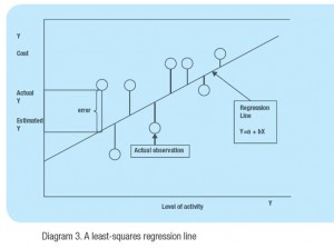
Least-squares regression is a statistical technique that uses all of the available data to find the best fitting line for a set of data points. This regression line, shown in Diagram (3), minimises the deviations of the actual Y values (the observed values of the cost) from the corresponding estimated Y values (the cost estimates) which lie along the regression line. These deviations are called the ‘estimation errors’. Some of these errors will be positive (where the estimated value of Y is greater than the observed value) while others will be negative (where the estimated value of Y is less than the observed value). Squaring all the negative errors produces a set of positive values which can then be added to the squared positive errors.
The regression line is the true line of best fit because the sum of all the squared errors is smaller for the regression line than for any other line that could be fitted to the data points. Hence this method is more accurate than all the other estimation methods, and we can utilise computer programs such as Excel to carry out the necessary calculations. Multiple regression analysis can be used when two or more independent variables (cost drivers) are assumed to influence a single dependent variable (a particular cost). In this case, there will be a separate regression coefficient (value of ‘b’) for each independent variable. Regression analysis also provides information about how well the regression line fits the data points. The coefficient of determination (or R squared value) indicates the proportion of the change in the Y (cost) values that is due to changes in the X (activity) values. An R squared value close to 1.0 shows that the regression model fits the data well, and we can be confident that cost predictions made using it will be fairly accurate.


